Linear Transformation and Matrices

Definition

A transformation is like a function. It ingests an input and spits an output. Ideally, transformations take ingest a vector and spit out another vector.

Why Not Call it a Function?

The main purpose of using transformation instead of a function is suggestive of a certain way to visualize the input/output relation. A great way to understand functions of vectors is to use movement.

If a transformation ingests an input vector and returns an output vector. We imagine the input vector moving over to the output vector.

We can imagine every single input vector moving over to its corresponding output vector. As we previously mentioned, it might be best to to visualize this concept with points instead of actual vector. Now instead of thinking of every possible input vector moving to its corresponding output vector. We can imagine very single input point, moving to its corresponding output point.

The “Linear” in Linear Transformation

A transformation is linear if it has two properties:

• All lines must remain lines, without getting curved.
• The Origin must remain fixed in place.

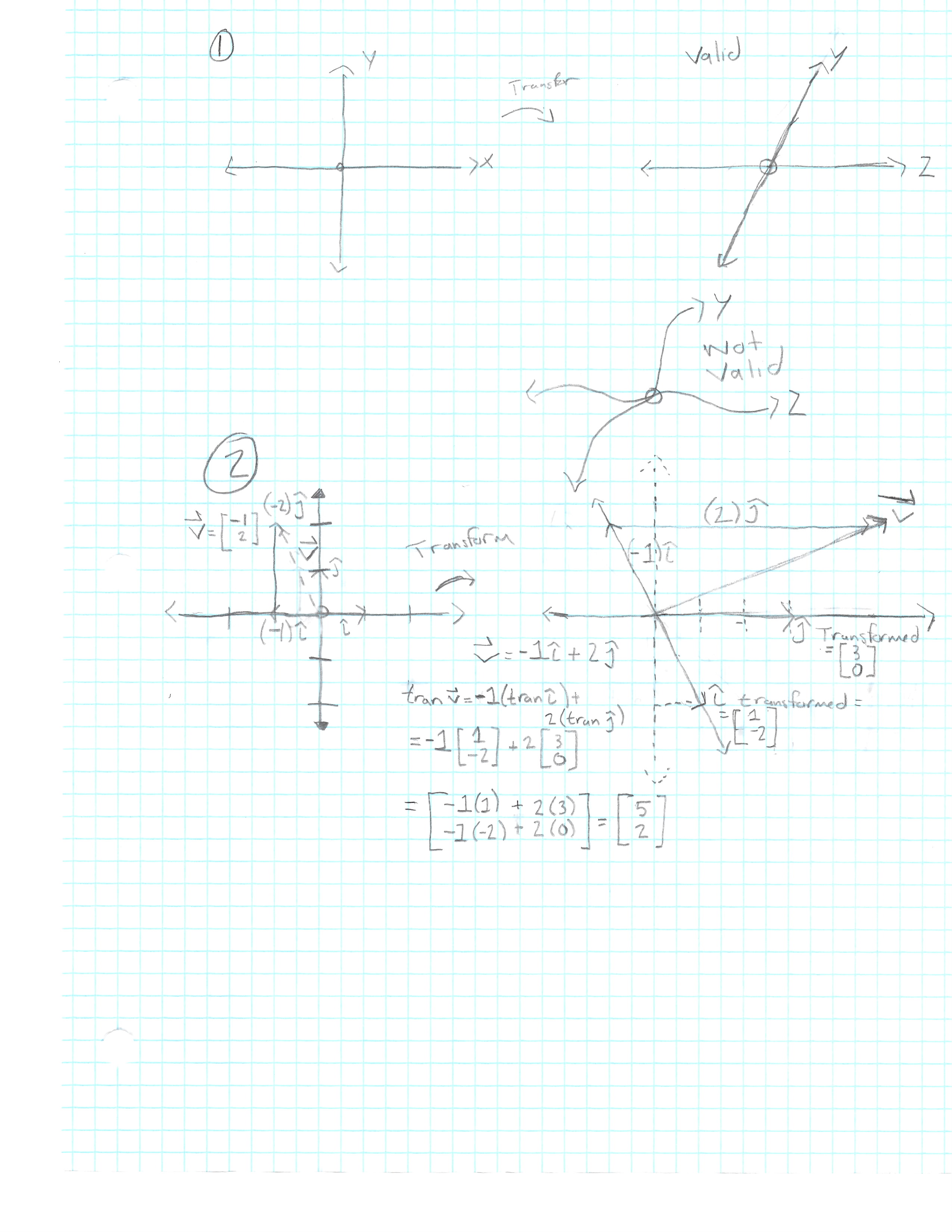
A general rule of thumb is, you should keep grid lines parallel and evenly spaced. (See image 1 below.)

Some transformations are easy to thing about. Such as rotations, others are harder to express with words.

Describing it Numerically

The questions then arises, “How can we express these transformations numerically”. So that you’re given the coordinates of an input vector, and able to transform and get the corresponding coordinates of the output vector.

It turns out, all you really need to do, is record where the basis vectors, i and j land. Everything else will simply follow from that.

(Follow image 2 below for the following)

If we start off with vector v at [-1, 2], transform it and follow the resulting vector. The resulting Vector v = (-1)*i* + (2)*j*. (Please picture the original grid underneath the new transformation)

In other words, it starts off as a linear combination of i and j, and it ends up as that same combination of where those basis vectors landed. This means you can deduce where v must go, based on where i and j land (keeping the original grid in the background helps the visualization here).

Now we can see that the transformed i = [1, -2], and transformed j = [3, 0].

Therefore if we follow the above equation

v = (-1)i + (2)j

 (-1)[ 1 ]   and   (2)[ 3 ]
     [-2 ]            [ 0 ]   

 [-1 ( 1 ) + 2 ( 3 )] = [ 5 ]
 [-1 (-2 ) + 2 ( 0 )]   [ 2 ]

Take a second, pause, and ponder.

Significance

By being able to visualize where i and j land, we can picture where v lands, without needing to draw it out.

i -> [ 1 ]   and   j -> [ 3 ]
     [-2 ]              [ 0 ]   

[ x ] -> (x) [ 1 ]  +  ( y ) [ 3 ]
[ y ]        [-2 ]           [ 0 ]  

This mean that a 2-D linear transformation is described by four numbers. The two coordinates for i and the two coordinates for j.

[1 ( x ) + 3 ( y )]
[-2( x ) + 0 ( y )]
     i         j

We can then package these numbers in a “2x2 Matrix”. Each column represents where i and j land. If you have a “2x2 Matrix” and a given input vector, you can calculate where that vector ends up, by adding the scale of the basis vectors.

[ 3  2 ]     [ 5 ]
[-2  1 ]     [ 7 ]

5[ 3 ]  +  7 [ 2 ]
 [-2 ]  +    [ 1 ]

The equation

Lets Imagine a matrix and a vector with letters.

  [ a   b ]    [ x ]
  [ c   d ]    [ y ]

This matrix is just another way of interpreting the linear transformation. The first column [ a c ] is where the first basis vector lands, while the second column [ b d ] is where the second basis vector lands. Now if you apply this linear transformation to the given vector. The result is the following:

[ a   b ][ x ]    x [ a ]  +  y [ b ]    =    [ ax  + by ]
[ c   d ][ y ]      [ c ]       [ d ]         [ bx  + dy ]

A major flaw in the way that linear algebra is commonly taught, is that you can easily teach someone this equation above, without exposing them to the crucial parts which makes this intuitive.

Practice Describing Vectors

• Rotate all of space 90 degrees counter clockwise. i -> [ 0 ] and j -> [-1 ] [ 1 ] [ 0 ]

  [ 0  -1 ][ x ]
  [ 1   0 ][ y ]
  

• A popular transformation is known as the “shear”.

  • i stays the same while j transforms

    i -> [ 1 ]   and   j -> [ 1 ]
         [ 0 ]              [ 1 ]   
    
    [ 1   1 ][ x ]
    [ 0   1 ][ y ]
    

Linearly Dependent Columns

If the coordinates of i and j are linearly dependent. Then the linear transformation squishes all 2-D space onto the line where those 2 vectors sit. Also known as the span of the two linearly dependent vectors.

Conclusion

Linear transformation is a way to move around space so that grid line remain parallel and evenly space, yet the origin stays the same. These transformations can be described using the coordinates of the basis vectors. Matrices give us a language to describe these transformations. Matrix vector multiplication is just a way to compute what a transformation does to a given vector.

The important takeaway is that every time you see a matrix, you can interpret what it does to any given vector.